It is important to note that the equations of motion only apply to an object that is moving with a constant acceleration. If the acceleration a was changing, you wouldn’t know what value to put in the equations.
Constant acceleration is often referred to as uniform acceleration.
The velocity–time graph in Figure 2.18 shows non-uniform acceleration. It is not a straight line; its gradient is changing (in this case, decreasing).

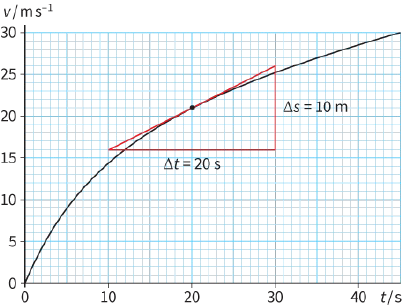
The acceleration at any instant in time is given by the gradient of the velocity–time graph. The triangle in Figure 2.18 shows how to find the acceleration at $t = 20$ seconds:
- At the time of interest, mark a point on the graph.
- Draw a tangent to the curve at that point.
Make a large right-angled triangle, and use it to find the gradient.
You can find the change in displacement of the body as it accelerates by determining the area under the velocity–time graph. 
To find the displacement of the object in Figure 2.18 between $t = 0$ and $t = 20 s$, the most straightforward, but lengthy, method is just to count the number of small squares.
In this case, up to $t = 20 s$, there are about 250 small squares. This is tedious to count but you can save yourself a lot of time by drawing a line from the origin to the point at $20 s$. The area of the triangle is easy to find (200 small squares) and then you only have to count the number of small squares between the line
you have drawn and the curve on the graph (about 50 squares)
In this case, each square is $1\,m\,{s^{ - 1}}$ on the y-axis by $1 s$ on the x-axis, so the area of each square is $1 \times 1 = 1m$ and the displacement is $250 m$. In other cases, note carefully the value of each side of the square you have chosen.

Questions

 

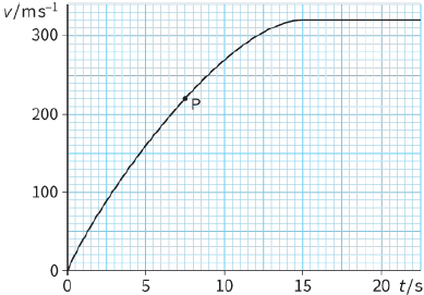
14) The graph in Figure 2.19 represents the motion of an object moving with varying acceleration. Lay your ruler on the diagram so that it is tangential to the graph at point P.
a: What are the values of time and velocity at this point?
b: Estimate the object’s acceleration at this point.

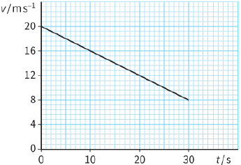
15) The velocity–time graph (Figure 2.20) represents the motion of a car along a straight road for a period of $30 s$.
a: Describe the motion of the car.
b: From the graph, determine the car’s initial and final velocities over the time of $30 s$.
c: Determine the acceleration of the car.
d: By calculating the area under the graph, determine the displacement of the car.
e: Check your answer to part d by calculating the car’s displacement using.